tcrClustR Workflow: TCR Clustering and Analysis

Introduction

The tcrClustR package provides tools for analyzing T-cell receptor (TCR) data by computing distance matrices between TCRs and clustering them into families. This vignette is the consolidated, primary guide and emphasizes the core production workflow:

CalculateTcrDistances() → RunTcrClustering()

It demonstrates the complete workflow using example data from the Rhesus Immunome Reference Atlas (https://bimberlab.github.io/RIRA/). Secondary sections outline the functions chained within RunTcrClustering() and their purposes.

Setup

First, we load the required libraries and set up the analysis parameters:


library(tcrClustR)
library(Seurat)

Load Example Data

We’ll use the example dataset included with the package:

# Load example Seurat object with TCR data
data_path <- system.file("extdata", "small_RIRA.rds", package = "tcrClustR")
seuratObj <- readRDS(data_path)

print("Seurat object summary:")
#> [1] "Seurat object summary:"
print(paste0("Number of cells: ", ncol(seuratObj)))
#> [1] "Number of cells: 4500"
print(paste0("Number of features: ", nrow(seuratObj)))
#> [1] "Number of features: 34606"

# Check for required TCR columns
tcr_columns <- c("TRA", "TRB", "TRA_V", "TRA_J", "TRB_V", "TRB_J")
available_tcr_cols <- intersect(tcr_columns, colnames(seuratObj@meta.data))
print(paste0("Available TCR columns: ", paste(available_tcr_cols, collapse = ", ")))
#> [1] "Available TCR columns: TRA, TRB, TRA_V, TRA_J, TRB_V, TRB_J"

Primary Workflow

1: Compute TCR Distance Matrices

This will take the TCR CDR3/V/J information (either stored in the seuratObj metadata or as a dataframe) and compute pairwise distances using tcrdist3:


seuratObj_TCR <- CalculateTcrDistances(
  inputData = seuratObj,
  chains = c("TRA", "TRB"),
  minimumCloneSize = 2,
  calculateChainPairs = TRUE
)
#> Warning in .flag_valid_rows(metadata = metadata, chains = chains, organism =
#> organism, : The following 15 TRA_V values were not found in the DB:
#> TRAV14-2,TRAV22-1,TRAV22-2,TRAV22-3,TRAV23-1,TRAV23-3,TRAV23-4,TRAV24-1,TRAV25-1,TRAV26-3,TRAV29,TRAV36,TRAV38-2,TRAV8-5,TRDV1-1.
#> Run tcrClustR:::.PullTcrdist3Db(organism = 'human', outputFilePath = '...') to
#> obtain the list of known segments.
#> Warning in .flag_valid_rows(metadata = metadata, chains = chains, organism =
#> organism, : The following 11 TRB_V values were not found in the DB:
#> TRBV2-1,TRBV2-2,TRBV2-3,TRBV3-3,TRBV3-4,TRBV5-10,TRBV5-9,TRBV6-2-1,TRBV7-10,TRBV7-5,TRBV7-7-1.
#> Run tcrClustR:::.PullTcrdist3Db(organism = 'human', outputFilePath = '...') to
#> obtain the list of known segments.
#> Preparing chain: TRA
#> Initial rows: 4500, after dropping invalid clones: 1877
#> Rows remaining after filtering clones with cloneSize less than 2: 73 (total dropped: 1804)
#> Unique metadata rows after grouping: 28
#> Preparing chain: TRB
#> Initial rows: 4500, after dropping invalid clones: 2748
#> Rows remaining after filtering clones with cloneSize less than 2: 139 (total dropped: 2609)
#> Unique metadata rows after grouping: 51
#> Calculating joint-chain distances
#> Calculating joint distance matrix for: TRA and TRB
#> TRA_TRB_fl, total passing cells: 1283
#> Total valid chain 1 clones: 26
#> Total valid chain 2 clones: 29
#> Calculating joint distance matrix for: TRA and TRB
#> TRA_TRB_cdr3, total passing cells: 1283
#> Total valid chain 1 clones: 26
#> Total valid chain 2 clones: 29

print("TCR distance matrices computed successfully!")
#> [1] "TCR distance matrices computed successfully!"
print(paste0("Available assays: ", paste(SeuratObject::Assays(seuratObj_TCR), collapse = ", ")))
#> [1] "Available assays: RNA"
print(paste0("Number of cells in TCR object: ", ncol(seuratObj_TCR)))
#> [1] "Number of cells in TCR object: 4500"

2: Cluster TCRs

Now we cluster the TCRs based on their similarity using DIANA (hierarchical) clustering. The resulting seurat object contains the raw distance matrices under the @misc slot. Cells are assigned to a family/cluster index for each chain:


seuratObj_TCR <- RunTcrClustering(
  seuratObj_TCR = seuratObj_TCR,
  dianaHeight = 20, 
  clusterSizeThreshold = 1
)
#> Processing assay: TRA_cdr3
#> Running DIANA clustering with cutHeight = 20
#> DIANA clustering produced 20 clusters
#> Thresholding clusters with minimum size = 1
#> Removed 0 clusters with < 1 clones
#> Total clones removed: 0
#> Remaining clusters: 20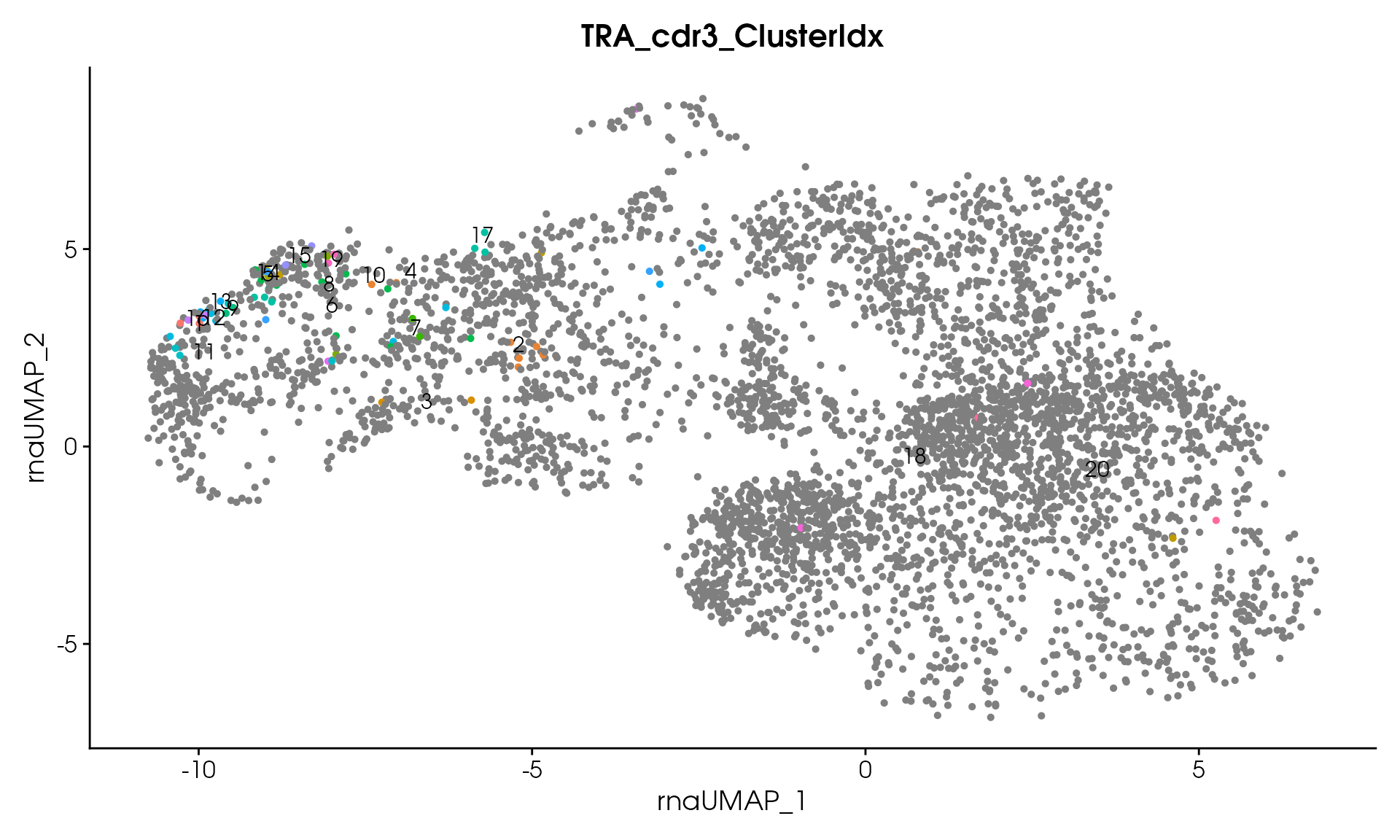

#> Processing assay: TRA_fl
#> Running DIANA clustering with cutHeight = 20
#> DIANA clustering produced 28 clusters
#> Thresholding clusters with minimum size = 1
#> Removed 0 clusters with < 1 clones
#> Total clones removed: 0
#> Remaining clusters: 28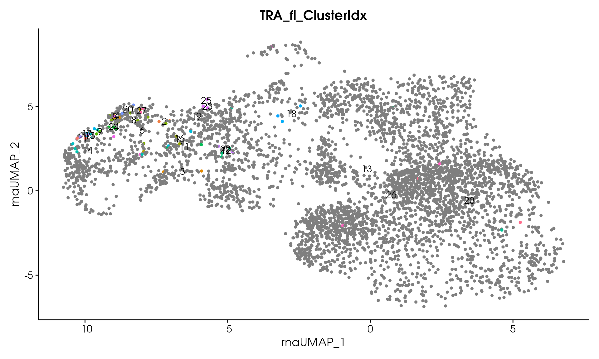

#> Processing assay: TRA_TRB_cdr3
#> Running DIANA clustering with cutHeight = 20
#> DIANA clustering produced 21 clusters
#> Thresholding clusters with minimum size = 1
#> Removed 0 clusters with < 1 clones
#> Total clones removed: 0
#> Remaining clusters: 21

#> Processing assay: TRA_TRB_fl
#> Running DIANA clustering with cutHeight = 20
#> DIANA clustering produced 21 clusters
#> Thresholding clusters with minimum size = 1
#> Removed 0 clusters with < 1 clones
#> Total clones removed: 0
#> Remaining clusters: 21

#> Processing assay: TRB_cdr3
#> Running DIANA clustering with cutHeight = 20
#> DIANA clustering produced 33 clusters
#> Thresholding clusters with minimum size = 1
#> Removed 0 clusters with < 1 clones
#> Total clones removed: 0
#> Remaining clusters: 33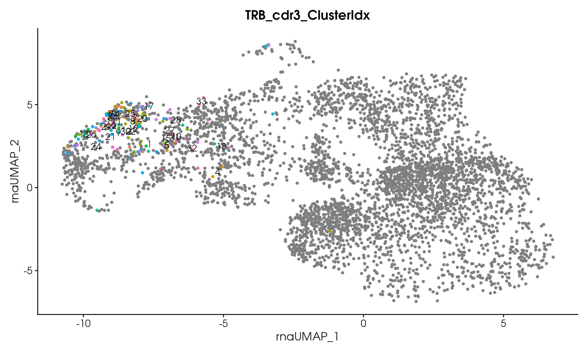

#> Processing assay: TRB_fl
#> Running DIANA clustering with cutHeight = 20
#> DIANA clustering produced 51 clusters
#> Thresholding clusters with minimum size = 1
#> Removed 0 clusters with < 1 clones
#> Total clones removed: 0
#> Remaining clusters: 51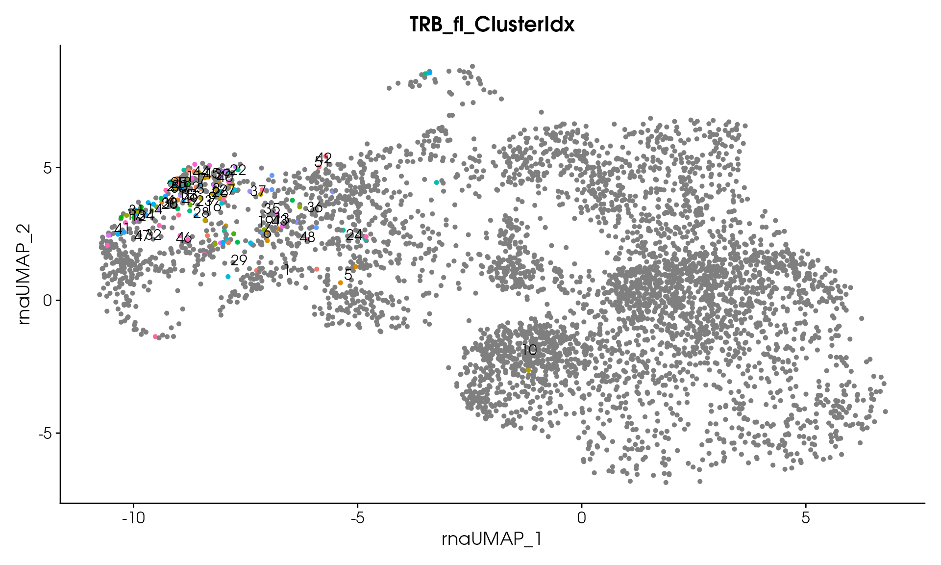


print("TCR clustering completed successfully!")
#> [1] "TCR clustering completed successfully!"


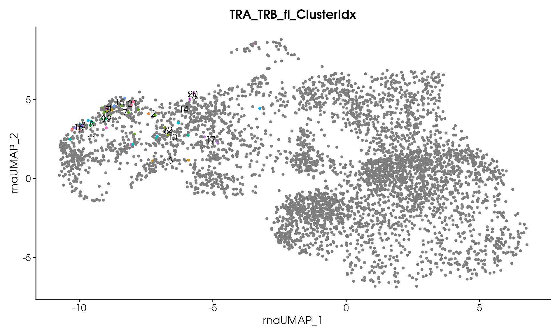
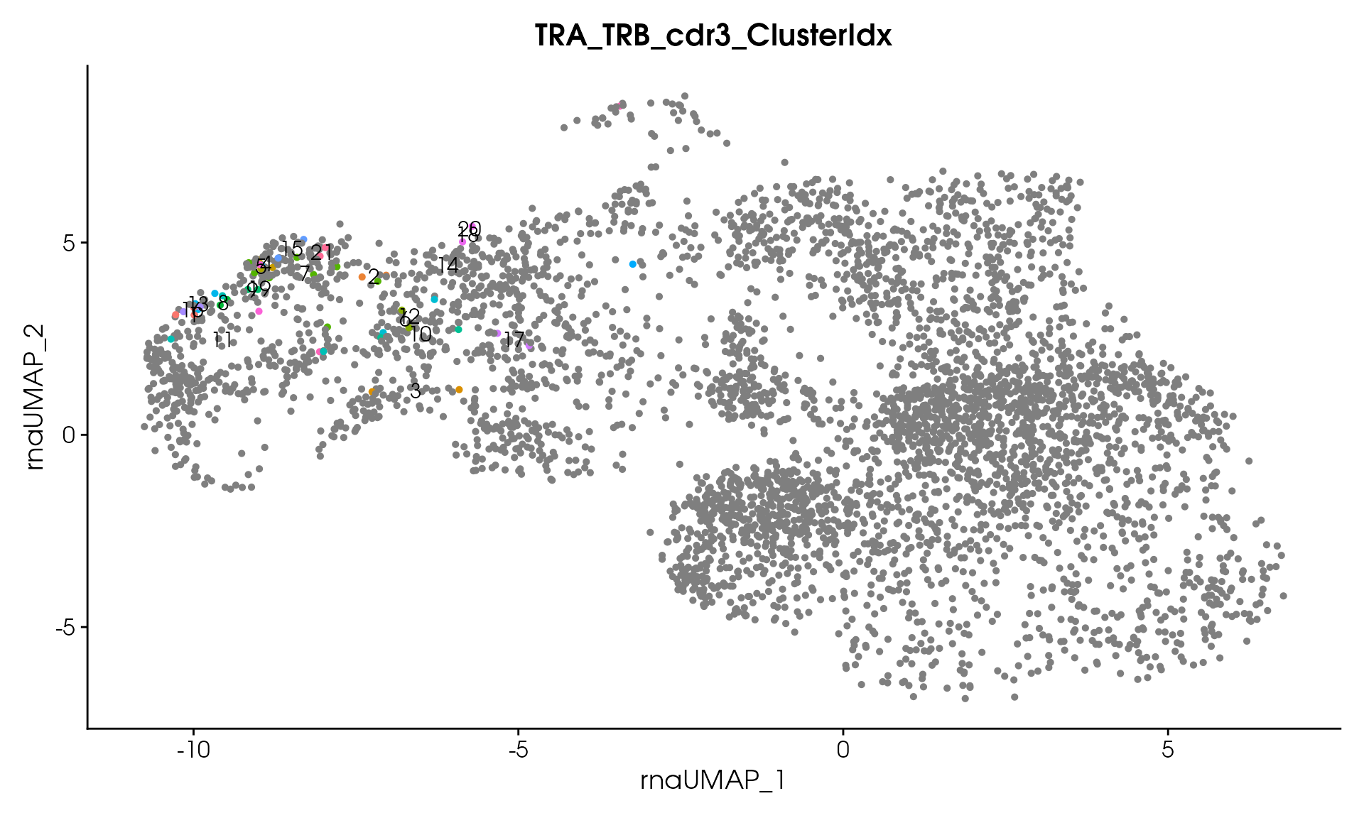
# Visualize
VisualizeTcrDistances(seuratObj_TCR)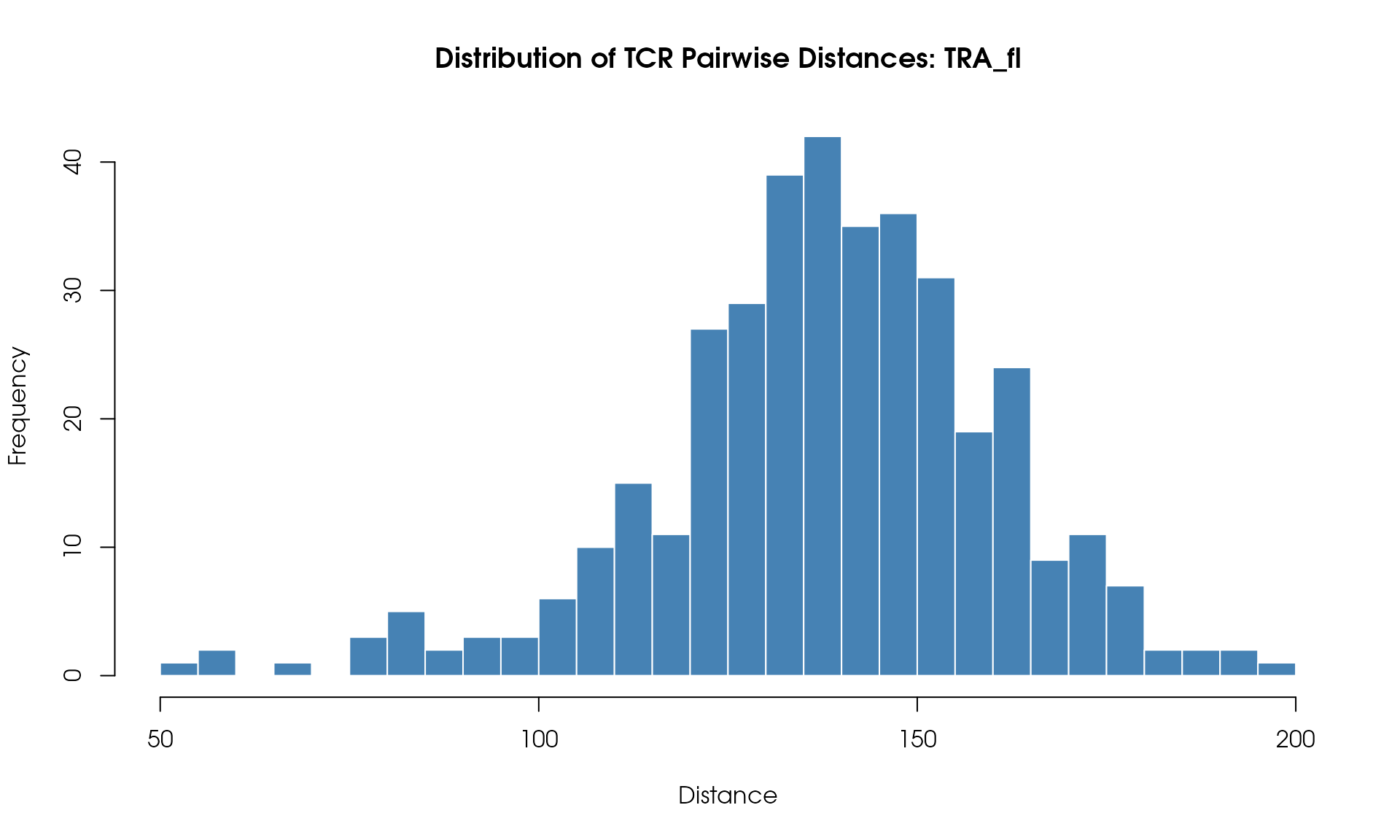

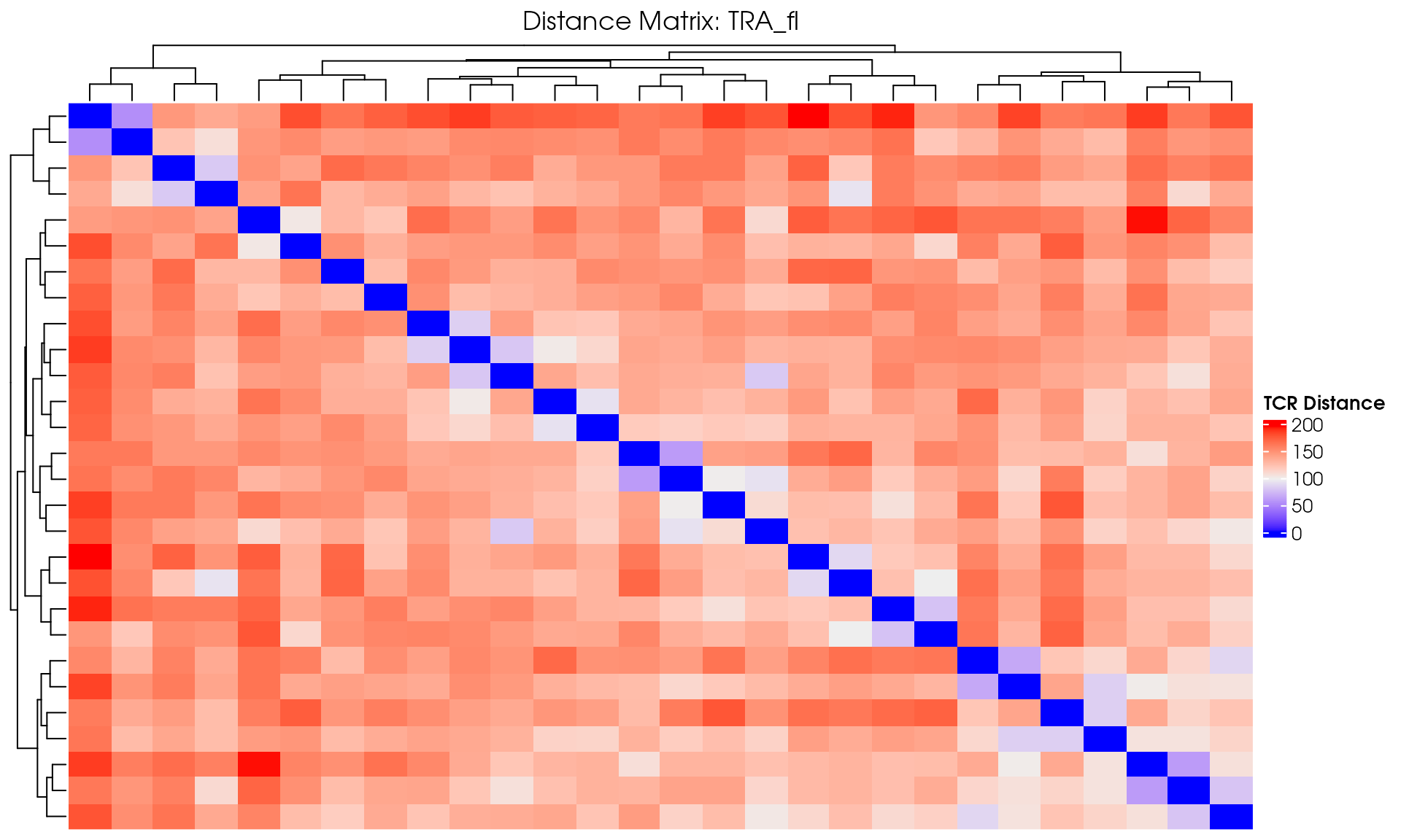
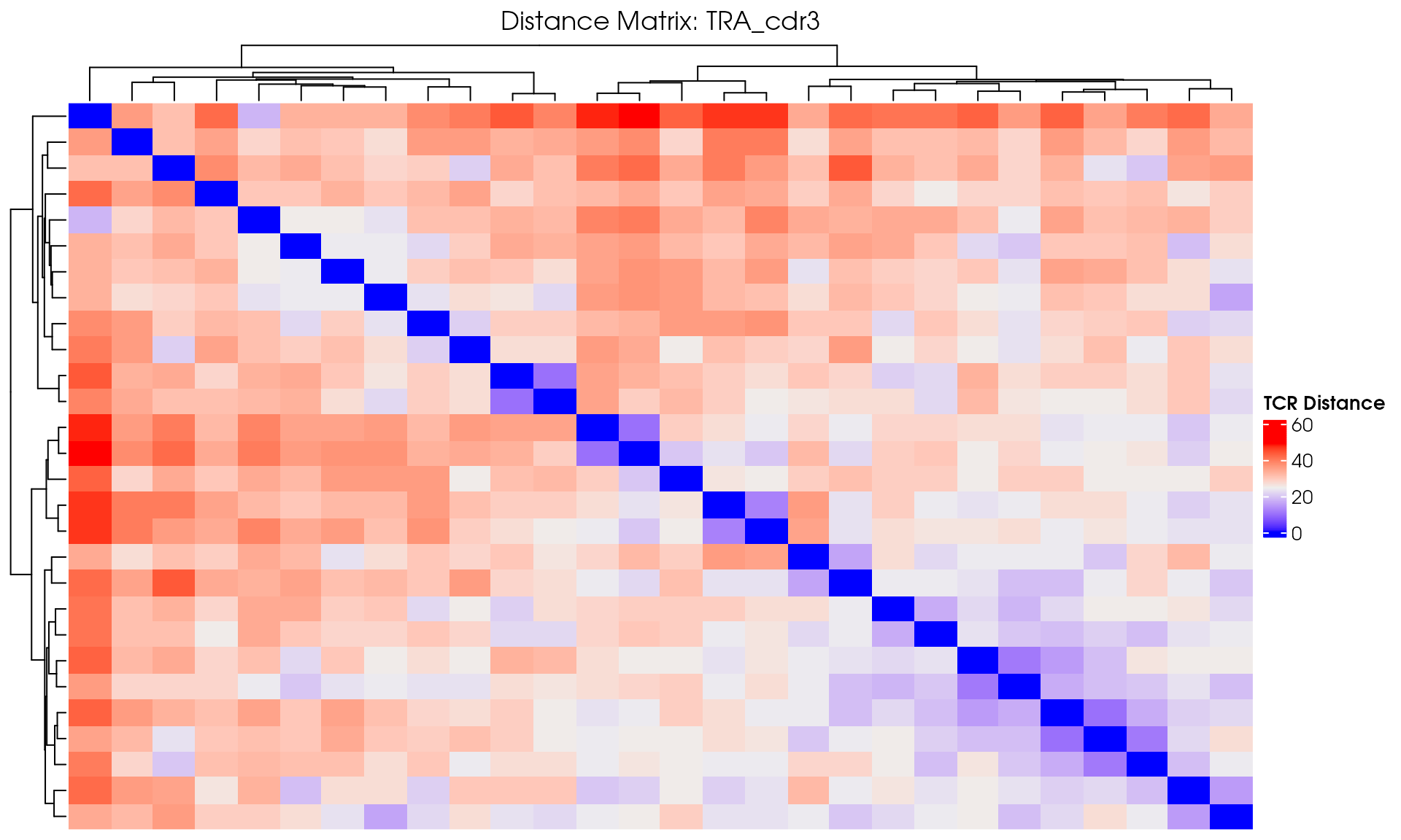
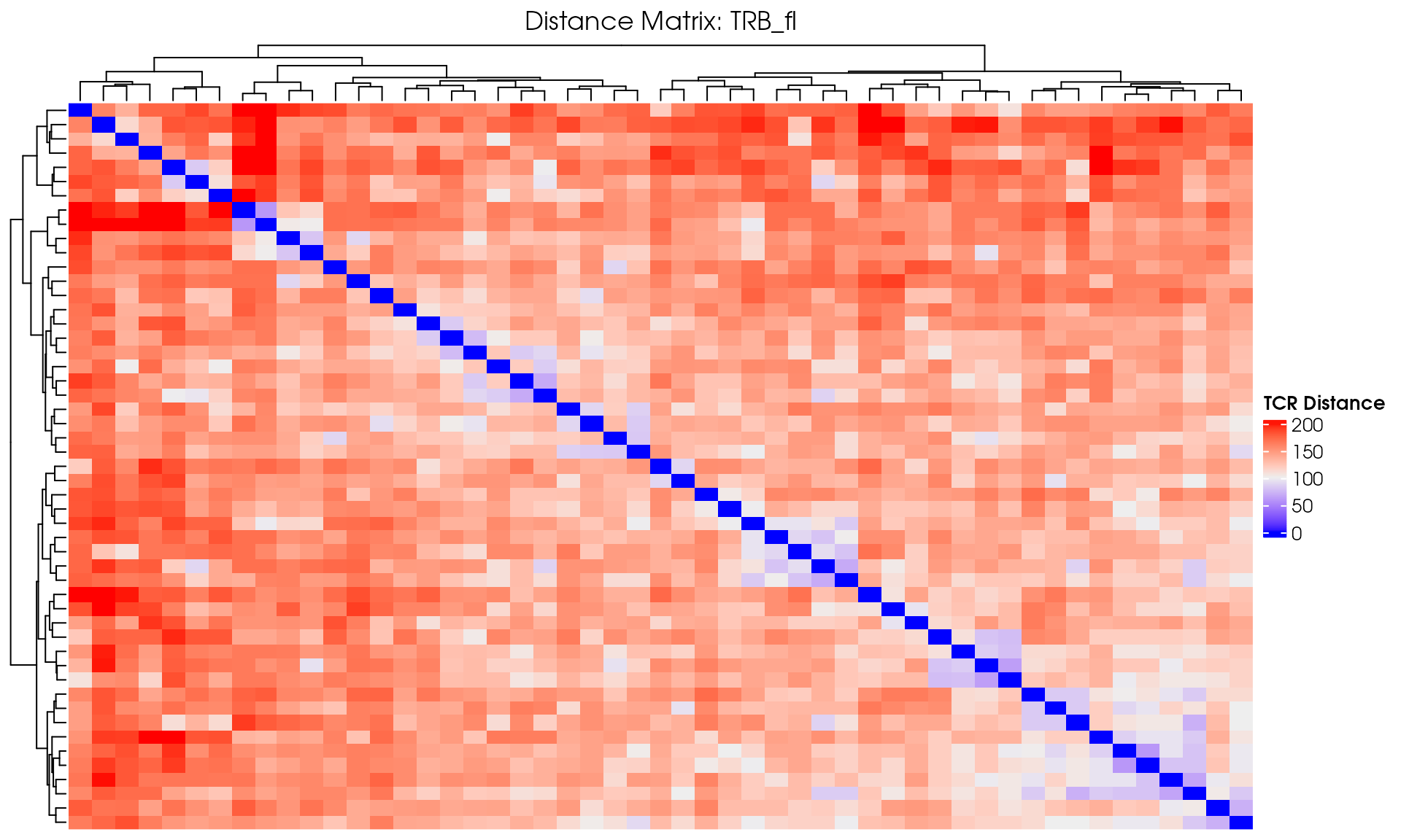
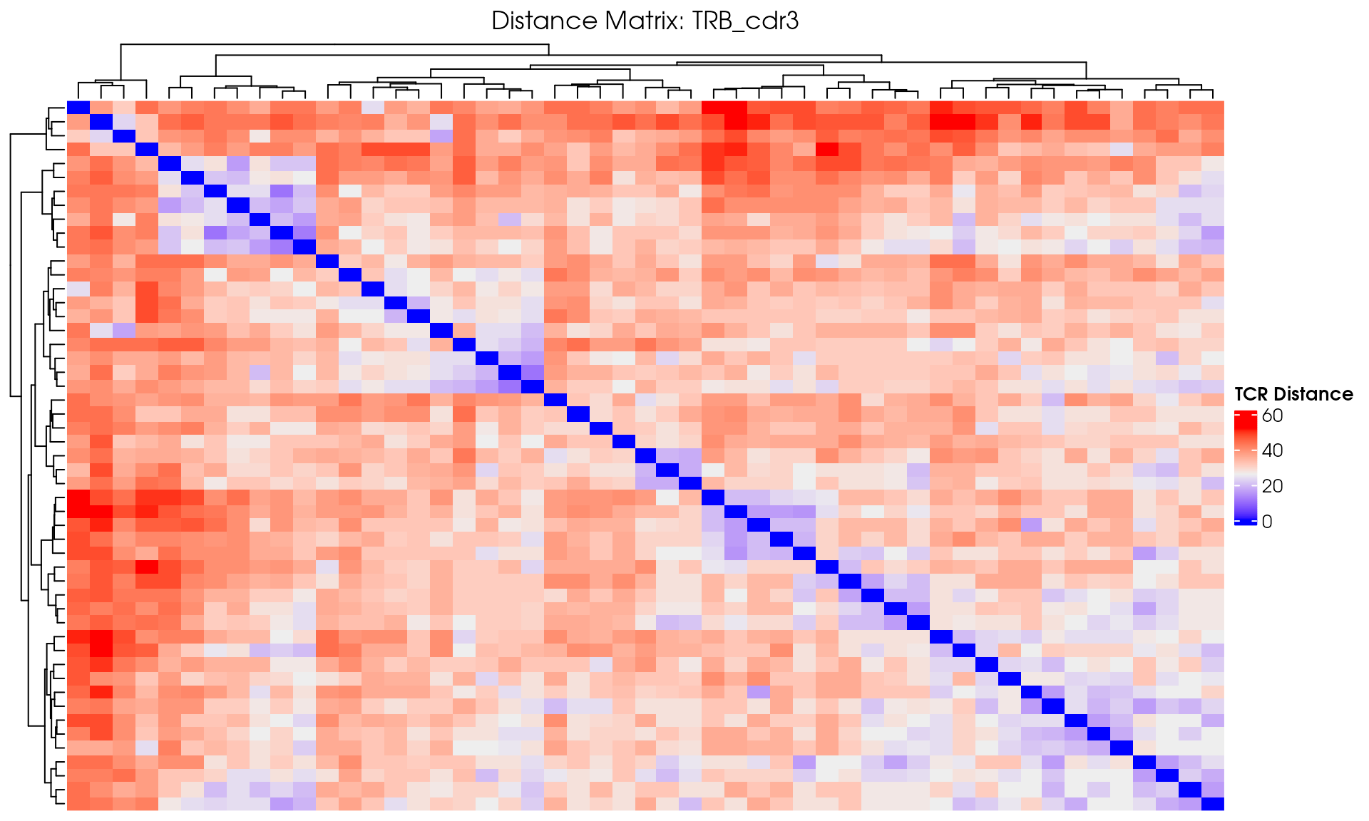
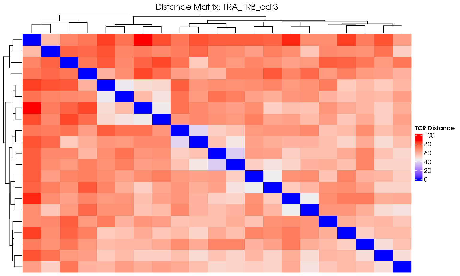
Visualize TCR Distance Matrices

After computing distance matrices with CalculateTcrDistances(), you can visualize the pairwise distances between TCR clones. The distance matrices are stored as Seurat assays in seuratObj_TCR.

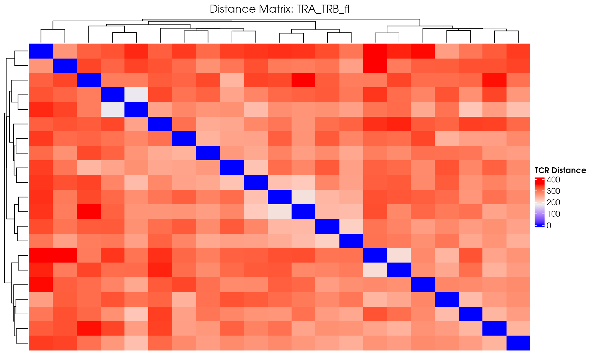
Basic Distance Heatmap

Create a simple heatmap showing TCR distances with hierarchical clustering:

library(ComplexHeatmap)
#> Loading required package: grid
#> ========================================
#> ComplexHeatmap version 2.26.1
#> Bioconductor page: http://bioconductor.org/packages/ComplexHeatmap/
#> Github page: https://github.com/jokergoo/ComplexHeatmap
#> Documentation: http://jokergoo.github.io/ComplexHeatmap-reference
#> 
#> If you use it in published research, please cite either one:
#> - Gu, Z. Complex Heatmap Visualization. iMeta 2022.
#> - Gu, Z. Complex heatmaps reveal patterns and correlations in multidimensional 
#>     genomic data. Bioinformatics 2016.
#> 
#> 
#> The new InteractiveComplexHeatmap package can directly export static 
#> complex heatmaps into an interactive Shiny app with zero effort. Have a try!
#> 
#> This message can be suppressed by:
#>   suppressPackageStartupMessages(library(ComplexHeatmap))
#> ========================================

# Extract distance matrix for TRB assay
distance_matrix <- GetDistanceMatrix(seuratObj_TCR, chains = "TRB")

# Create a hierarchical clustered heatmap
distance_heatmap <- ComplexHeatmap::Heatmap(
  as.matrix(distance_matrix),
  name = "TCR Distance",
  show_row_names = FALSE,
  show_column_names = FALSE,
  cluster_rows = TRUE,
  cluster_columns = TRUE,
  clustering_method_rows = "ward.D2",
  clustering_method_columns = "ward.D2",
  use_raster = TRUE,
  show_heatmap_legend = TRUE,
  column_title = "TRB Distance Matrix"
)

draw(distance_heatmap)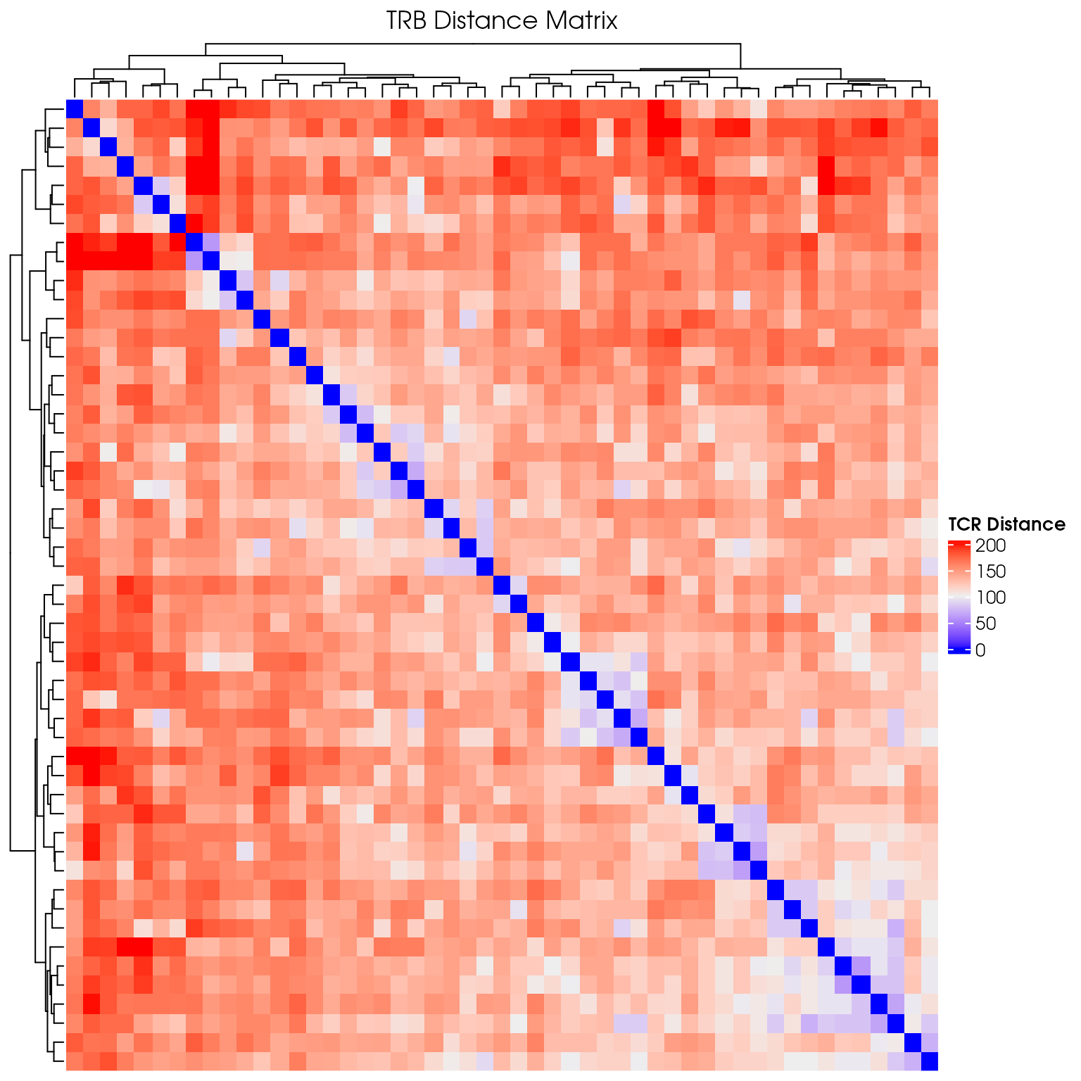

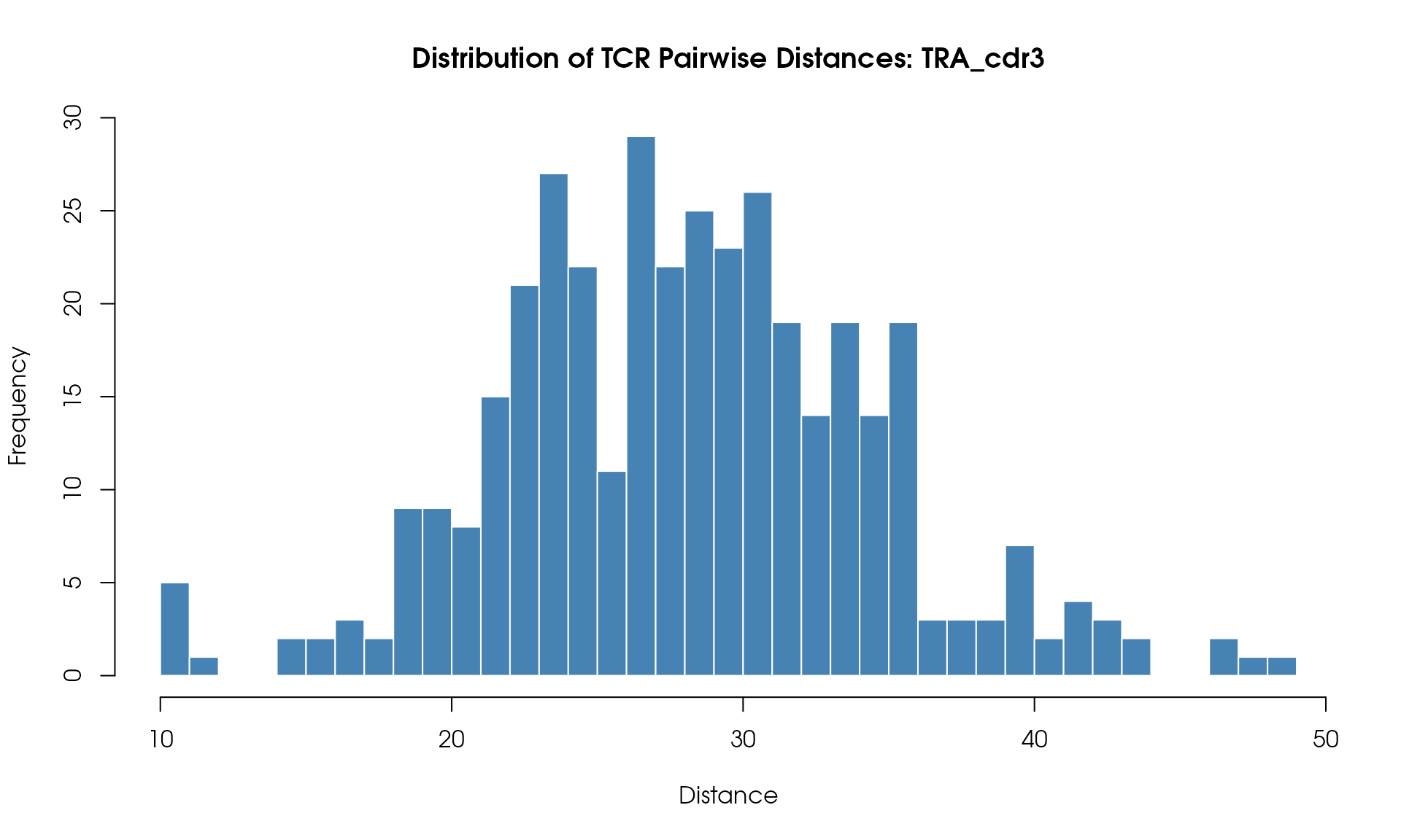
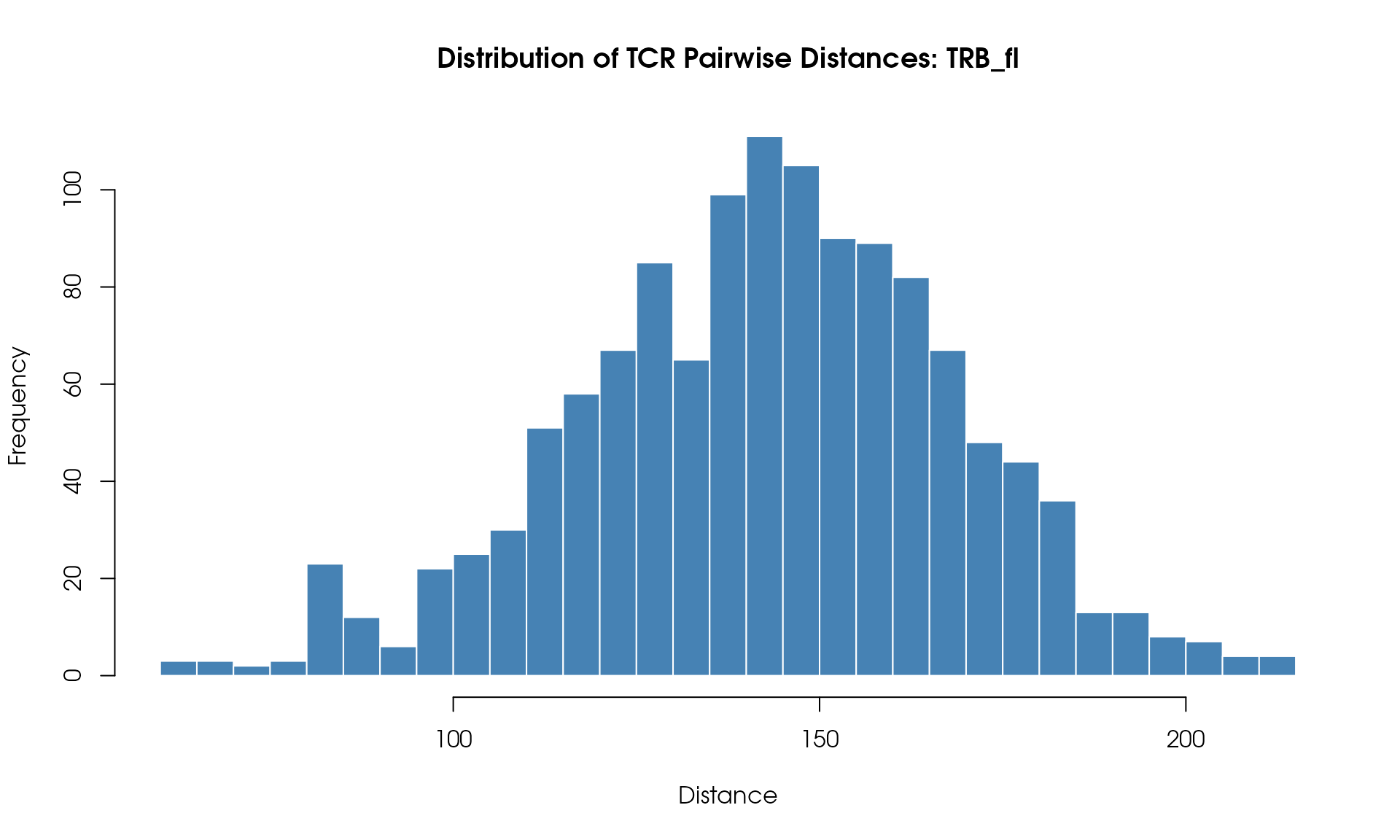
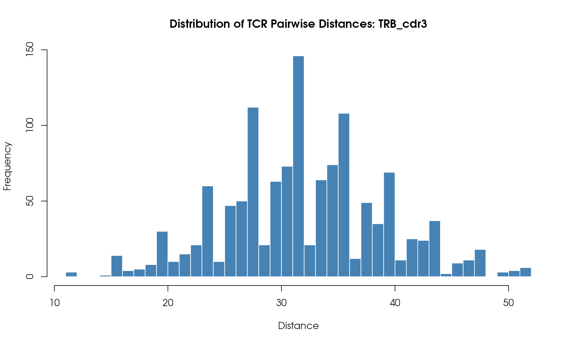
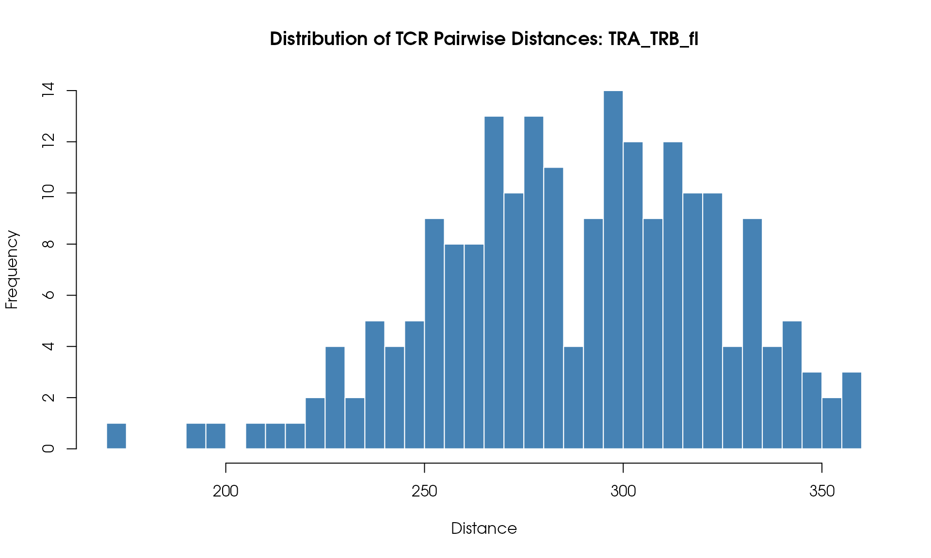
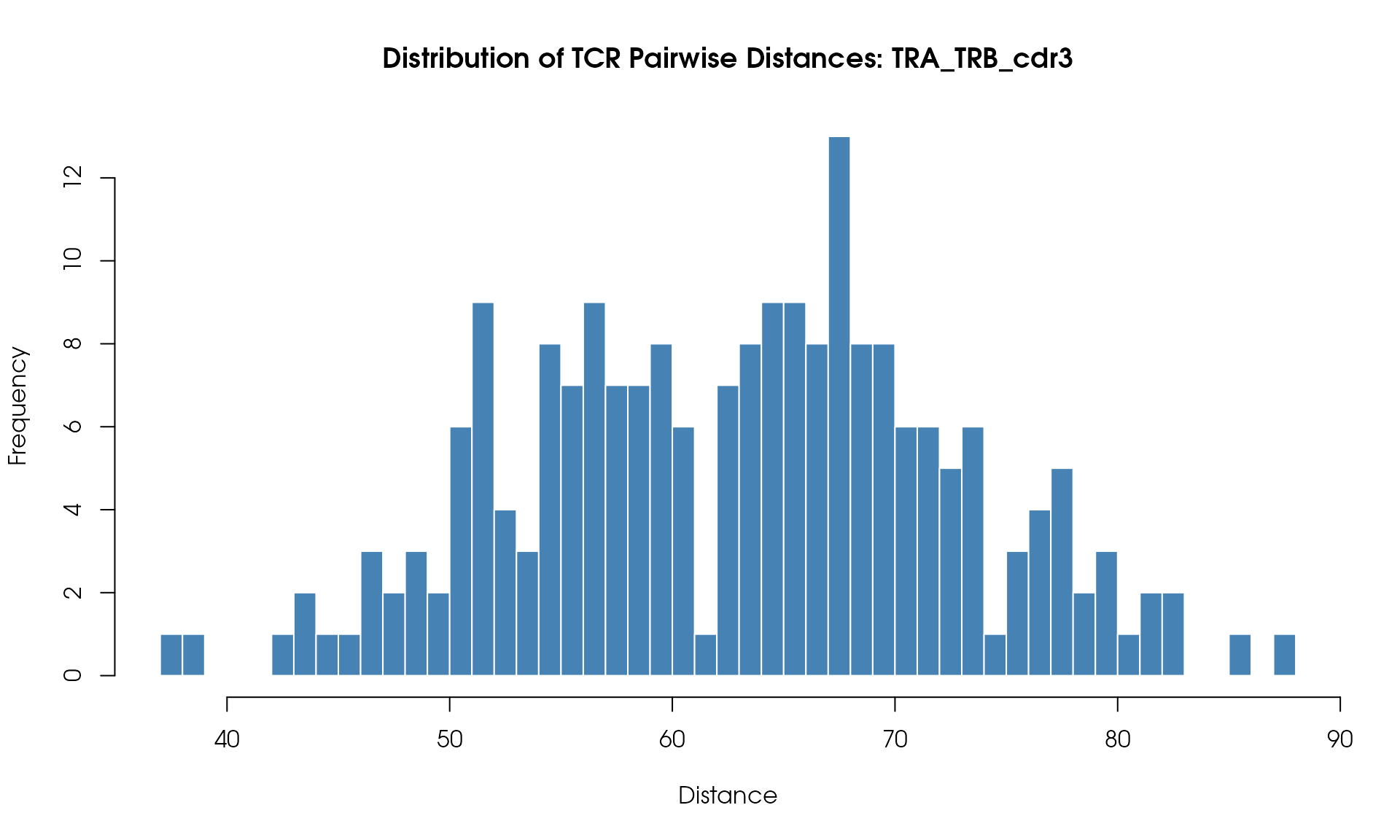
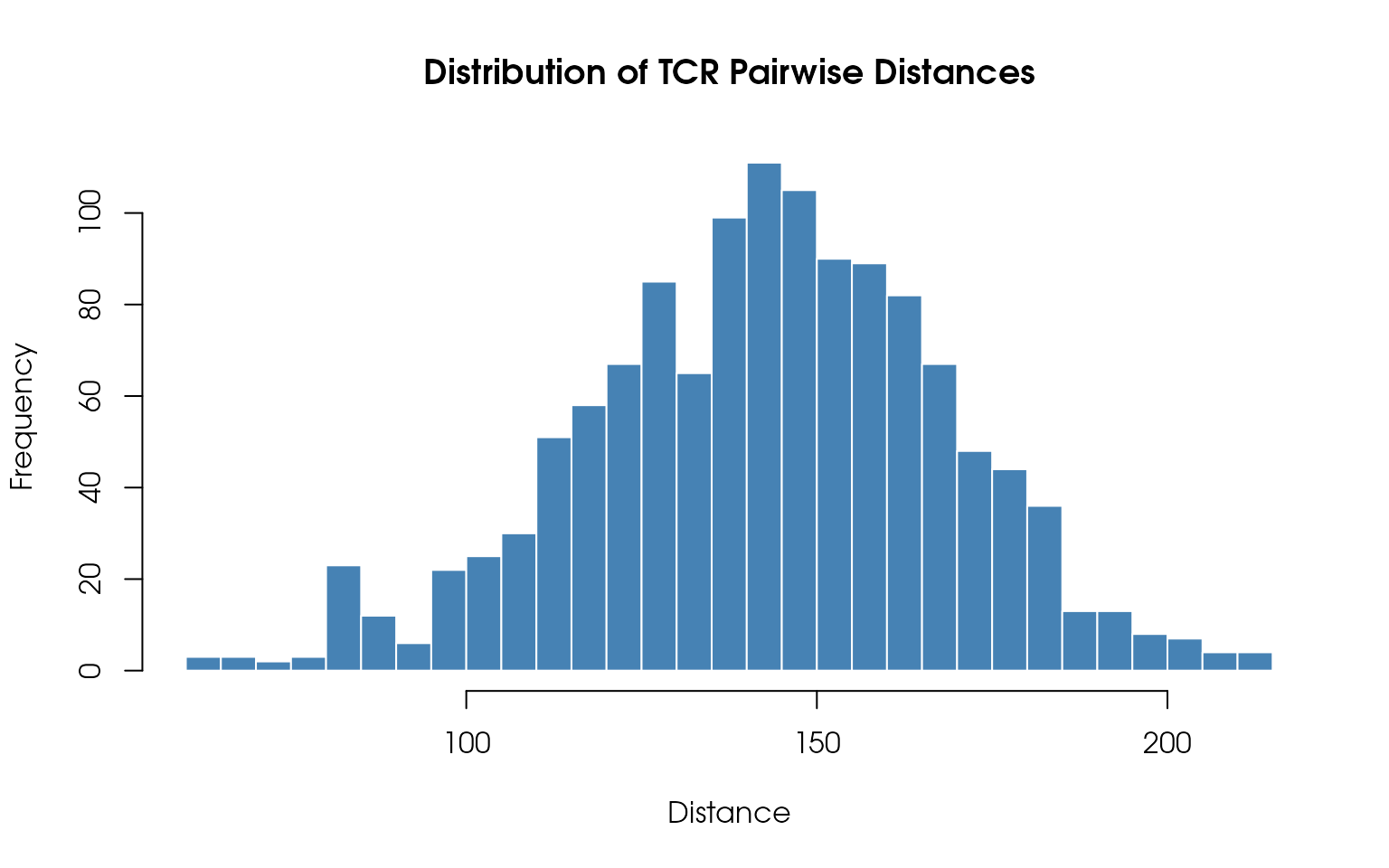
Distance Histogram

Visualize the distribution of pairwise TCR distances:

# Extract upper triangle of distance matrix (avoid duplicates)
dist_values <- distance_matrix[upper.tri(distance_matrix)]

# Plot histogram
hist(
  dist_values,
  breaks = 50,
  main = "Distribution of TCR Pairwise Distances",
  xlab = "Distance",
  ylab = "Frequency",
  col = "steelblue",
  border = "white"
)

Understanding the Results

The tcrClustR workflow produces several key outputs:

Distance Matrices: Pairwise distances between TCRs based on various metrics
Clustering Results: TCRs grouped into clusters based on similarity
Visualizations: Heatmaps and histograms showing clustering patterns
Clonotypic Join: Transfer of clustering results back to the original Seurat object

Interpreting Clusters

Each cluster represents a group of similar TCRs that may have related functions
Cluster assignments are added as new columns to your Seurat object metadata after the clonotypic join
Cells without TCR data will have NA values for clustering columns

Next Steps

With clustering results now available in your main Seurat object, you can:

Analyze cluster composition: Examine which cell types or conditions are enriched in each TCR cluster
Functional analysis: Investigate whether TCR clusters correlate with specific cellular functions
Comparative studies: Compare TCR clustering patterns across different experimental conditions
Integration with other data: Combine TCR clustering with gene expression, surface marker, or other omics data

The resolution parameter controls the granularity of clustering (lower = fewer, larger clusters)

Next Steps

After clustering, you can:

Extract specific clusters for further analysis
Use cluster assignments for downstream functional studies
Prioritize representative TCRs from each cluster for synthesis
Correlate clusters with phenotypic or functional data

Session Information

sessionInfo()
#> R version 4.5.2 (2025-10-31)
#> Platform: x86_64-pc-linux-gnu
#> Running under: Debian GNU/Linux trixie/sid
#> 
#> Matrix products: default
#> BLAS:   /usr/lib/x86_64-linux-gnu/openblas-pthread/libblas.so.3 
#> LAPACK: /usr/lib/x86_64-linux-gnu/openblas-pthread/libopenblasp-r0.3.28.so;  LAPACK version 3.12.0
#> 
#> locale:
#>  [1] LC_CTYPE=en_US.UTF-8       LC_NUMERIC=C              
#>  [3] LC_TIME=en_US.UTF-8        LC_COLLATE=en_US.UTF-8    
#>  [5] LC_MONETARY=en_US.UTF-8    LC_MESSAGES=en_US.UTF-8   
#>  [7] LC_PAPER=en_US.UTF-8       LC_NAME=C                 
#>  [9] LC_ADDRESS=C               LC_TELEPHONE=C            
#> [11] LC_MEASUREMENT=en_US.UTF-8 LC_IDENTIFICATION=C       
#> 
#> time zone: Etc/UTC
#> tzcode source: system (glibc)
#> 
#> attached base packages:
#> [1] grid      stats     graphics  grDevices utils     datasets  methods  
#> [8] base     
#> 
#> other attached packages:
#> [1] ComplexHeatmap_2.26.1 Seurat_5.4.0.9009     SeuratObject_5.3.0   
#> [4] sp_2.2-1              tcrClustR_0.0.0.9003 
#> 
#> loaded via a namespace (and not attached):
#>   [1] RColorBrewer_1.1-3     jsonlite_2.0.0         shape_1.4.6.1         
#>   [4] magrittr_2.0.4         magick_2.9.1           spatstat.utils_3.2-1  
#>   [7] farver_2.1.2           rmarkdown_2.30         GlobalOptions_0.1.3   
#>  [10] fs_1.6.7               ragg_1.5.1             vctrs_0.7.1           
#>  [13] ROCR_1.0-12            spatstat.explore_3.7-0 htmltools_0.5.9       
#>  [16] sass_0.4.10            sctransform_0.4.3      parallelly_1.46.1     
#>  [19] KernSmooth_2.23-26     bslib_0.10.0           htmlwidgets_1.6.4     
#>  [22] desc_1.4.3             ica_1.0-3              plyr_1.8.9            
#>  [25] plotly_4.12.0          zoo_1.8-15             cachem_1.1.0          
#>  [28] igraph_2.2.2           mime_0.13              lifecycle_1.0.5       
#>  [31] iterators_1.0.14       pkgconfig_2.0.3        Matrix_1.7-4          
#>  [34] R6_2.6.1               fastmap_1.2.0          fitdistrplus_1.2-6    
#>  [37] future_1.69.0          shiny_1.13.0           clue_0.3-67           
#>  [40] digest_0.6.39          colorspace_2.1-2       dirichletprocess_0.4.2
#>  [43] patchwork_1.3.2        S4Vectors_0.48.0       tensor_1.5.1          
#>  [46] RSpectra_0.16-2        irlba_2.3.7            textshaping_1.0.5     
#>  [49] labeling_0.4.3         progressr_0.18.0       spatstat.sparse_3.1-0 
#>  [52] httr_1.4.8             polyclip_1.10-7        abind_1.4-8           
#>  [55] compiler_4.5.2         withr_3.0.2            bit64_4.6.0-1         
#>  [58] doParallel_1.0.17      S7_0.2.1               fastDummies_1.7.5     
#>  [61] R.utils_2.13.0         MASS_7.3-65            rjson_0.2.23          
#>  [64] tools_4.5.2            lmtest_0.9-40          otel_0.2.0            
#>  [67] httpuv_1.6.16          future.apply_1.20.2    goftest_1.2-3         
#>  [70] R.oo_1.27.1            glue_1.8.0             nlme_3.1-168          
#>  [73] promises_1.5.0         Rtsne_0.17             cluster_2.1.8.2       
#>  [76] reshape2_1.4.5         generics_0.1.4         gtable_0.3.6          
#>  [79] spatstat.data_3.1-9    tzdb_0.5.0             R.methodsS3_1.8.2     
#>  [82] tidyr_1.3.2            hms_1.1.4              data.table_1.18.2.1   
#>  [85] BiocGenerics_0.56.0    spatstat.geom_3.7-0    RcppAnnoy_0.0.23      
#>  [88] ggrepel_0.9.7          RANN_2.6.2             foreach_1.5.2         
#>  [91] pillar_1.11.1          stringr_1.6.0          vroom_1.7.0           
#>  [94] spam_2.11-3            RcppHNSW_0.6.0         later_1.4.8           
#>  [97] circlize_0.4.17        splines_4.5.2          dplyr_1.2.0           
#> [100] lattice_0.22-9         bit_4.6.0              survival_3.8-6        
#> [103] deldir_2.0-4           tidyselect_1.2.1       miniUI_0.1.2          
#> [106] pbapply_1.7-4          knitr_1.51             gridExtra_2.3         
#> [109] IRanges_2.44.0         scattermore_1.2        stats4_4.5.2          
#> [112] xfun_0.56              matrixStats_1.5.0      stringi_1.8.7         
#> [115] lazyeval_0.2.2         yaml_2.3.12            evaluate_1.0.5        
#> [118] codetools_0.2-20       tibble_3.3.1           cli_3.6.5             
#> [121] uwot_0.2.4             xtable_1.8-8           reticulate_1.45.0     
#> [124] systemfonts_1.3.2      jquerylib_0.1.4        Rcpp_1.1.1            
#> [127] spatstat.random_3.4-4  globals_0.19.0         png_0.1-8             
#> [130] spatstat.univar_3.1-6  parallel_4.5.2         readr_2.2.0           
#> [133] pkgdown_2.2.0          ggplot2_4.0.2          dotCall64_1.2         
#> [136] listenv_0.10.0         viridisLite_0.4.3      scales_1.4.0          
#> [139] ggridges_0.5.7         purrr_1.2.1            crayon_1.5.3          
#> [142] GetoptLong_1.1.0       rlang_1.1.7            cowplot_1.2.0

Conclusion

This vignette demonstrated the complete tcrClustR workflow for analyzing TCR data. The package provides a streamlined approach to:

Format TCR metadata for analysis
Compute distance matrices between TCRs
Cluster TCRs based on similarity
Visualize and interpret results

The resulting clusters can be used to identify groups of potentially functionally related TCRs for downstream analysis and experimental validation.

GW McElfresh, Sebastian Benjamin, & Bimber Lab

2026-03-10

Introduction

Setup

Load Example Data

Primary Workflow

1: Compute TCR Distance Matrices

2: Cluster TCRs

Visualize TCR Distance Matrices

Basic Distance Heatmap

Distance Histogram

Understanding the Results

Interpreting Clusters

Next Steps

Next Steps

Session Information

Conclusion